Here is an interesting blog post from Igor Carron,
which tries to answer my question: is it possible to implement a large scale randomized
SVD solver?
Wednesday, October 26, 2011
Saturday, October 22, 2011
Speeding up SVD on a mega matrix using GraphLab - part 2
It seems I struck some nerve, since I am getting a lot of comments about this blog post.
First, here is an email I got from Bryan, Research Programmer at CMU:
"The machine in question, named "thrust", features two Xeon X5690 CPUs. Each one has 12 hyperthreaded cores, clock speed 3.47GHz, 64 KB L1 cache/core (32 KB L1 Data + 32 KB L1 Instruction) and 256 KB L2 cache/core, and 12MB L3 cache. It's got 192GB of RAM. We're running Ubuntu 10.04 LTS with the Ubuntu-supplied underlying libraries (boost, ITPP, etc.), some of which are a bit older than the ones supplied to the newer version of Ubuntu mentioned on your blog.
No problem on getting you access to this machine. The only difficulty would be in coordinating who gets to use it when. We have other somewhat less well-endowed machines of identical hardware platform and software setup that see more idle time where it'd be easier to fit in runs that take only a few tens of GB of RAM and, say, half a dozen cores.
To elaborate on what I observed during Abhay's run, I present the following strage wall of numbers excerpted from a home-grown load monitoring script:
Fri-Oct-21-03:31:23 1319182283 13.2 3.0 0.0 7.6 0.1 0.6/ 13.2 0.0/12.4
Fri-Oct-21-03:31:28 1319182288 5.711.0 0.0 9.0 0.0 1.3/ 29.6 0.0/ 0.0
Fri-Oct-21-03:31:33 1319182293 6.7 1.7 0.016.5 0.0 1.3/ 30.0 0.0/ 0.0
Fri-Oct-21-03:31:38 1319182298 10.4 2.1 0.012.4 0.0 1.3/ 30.5 0.0/ 0.0
Fri-Oct-21-03:31:43 1319182303 6.8 8.8 0.0 9.1 0.0 1.8/ 31.2 0.0/14.0
Fri-Oct-21-03:31:48 1319182308 4.5 2.1 0.018.4 0.0 1.3/ 31.2 0.0/ 0.0
Fri-Oct-21-03:31:53 1319182313 1.9 1.2 0.021.6 0.0 1.3/ 30.1 0.0/ 0.0
Fri-Oct-21-03:31:58 1319182318 13.2 2.4 0.0 9.1 0.0 1.3/ 31.6 0.0/ 0.0
Fri-Oct-21-03:32:03 1319182323 5.211.8 0.0 7.7 0.0 1.4/ 36.5 0.0/ 0.0
Fri-Oct-21-03:32:08 1319182328 7.5 1.8 0.015.7 0.0 1.5/ 37.7 0.0/ 0.0
Fri-Oct-21-03:32:13 1319182333 9.7 1.6 0.013.8 0.0 2.2/ 33.0 0.0/ 0.0
Fri-Oct-21-03:32:18 1319182338 7.9 8.1 0.0 8.8 0.0 1.4/ 34.4 0.0/14.0
Fri-Oct-21-03:32:23 1319182343 4.5 2.1 0.018.3 0.0 1.5/ 37.3 0.0/ 0.0
Fri-Oct-21-03:32:28 1319182348 2.0 1.7 0.021.0 0.0 1.5/ 40.7 0.0/ 0.0
Fri-Oct-21-03:32:33 1319182353 13.2 2.1 0.0 9.7 0.0 1.6/ 42.3 0.0/ 0.0
Fri-Oct-21-03:32:38 1319182358 5.212.7 0.0 6.6 0.0 1.6/ 43.8 0.0/ 0.0
Fri-Oct-21-03:32:43 1319182363 8.1 2.1 0.014.7 0.0 6.7/ 24.8 0.0/ 0.0
Fri-Oct-21-03:32:48 1319182368 7.9 1.4 0.015.6 0.0 1.3/ 28.1 0.0/ 0.0
Fri-Oct-21-03:32:53 1319182373 8.8 8.9 0.0 7.1 0.0 1.3/ 28.3 0.0/14.0
Fri-Oct-21-03:32:58 1319182378 4.7 2.2 0.018.1 0.0 1.3/ 28.3 0.0/ 0.0
Fri-Oct-21-03:33:03 1319182383 2.4 1.2 0.021.2 0.0 1.3/ 28.0 0.0/ 0.0
Fri-Oct-21-03:33:08 1319182388 11.6 2.1 0.011.3 0.0 1.3/ 25.8 0.0/ 0.0
Fri-Oct-21-03:33:13 1319182393 6.212.5 0.0 5.7 0.0 2.0/ 27.9 0.0/ 0.0
Fri-Oct-21-03:33:18 1319182398 8.9 2.0 0.014.0 0.0 1.5/ 32.7 0.0/ 0.0
Fri-Oct-21-03:33:23 1319182403 6.2 1.8 0.016.8 0.0 1.3/ 30.6 0.0/ 0.0
Fri-Oct-21-03:33:28 1319182408 10.4 7.9 0.0 6.4 0.0 1.4/ 29.8 0.0/14.0
Fri-Oct-21-03:33:33 1319182413 4.6 2.1 0.018.4 0.0 1.4/ 29.8 0.0/ 0.0
Fri-Oct-21-03:33:38 1319182418 2.5 1.8 0.020.7 0.0 1.2/ 27.1 0.0/ 0.0
Fri-Oct-21-03:33:43 1319182423 10.1 1.8 0.013.1 0.0 1.9/ 23.8 0.0/ 0.0
Fri-Oct-21-03:33:48 1319182428 6.912.0 0.0 5.6 0.0 1.3/ 28.4 0.0/ 0.0
Fri-Oct-21-03:33:53 1319182433 8.9 1.7 0.014.3 0.0 1.5/ 35.6 0.0/ 0.0
Fri-Oct-21-03:33:58 1319182438 6.0 1.8 0.017.0 0.0 1.4/ 32.2 0.0/ 0.0
Fri-Oct-21-03:34:03 1319182443 10.3 8.7 0.0 5.6 0.0 1.4/ 35.1 0.0/14.0
Fri-Oct-21-03:34:09 1319182449 3.8 1.8 0.015.2 0.0 3.7/ 27.9 0.0/ 0.0
Fri-Oct-21-03:34:14 1319182454 2.9 1.8 0.020.1 0.0 1.2/ 26.9 0.0/ 0.0
Fri-Oct-21-03:34:19 1319182459 8.7 2.1 0.014.2 0.0 1.3/ 25.0 0.0/ 0.0
Each row represents some statistic averaged over the last five seconds. The first two columns are time stamps. The interesting bit is the next grouping with five columns of poorly-spaced numbers. The first number is the average number of cores doing something in the kernel. We see here that the process has spurts where it will spend ~10 cores in the kernel for ~five seconds, and then that number will back off for 15-30 seconds. The next column counts idle time, and we see a spike in idle time after each spike of kernel time, and that this spike is of similar or perhaps greater magnitude. The 3rd column is all zeros. The 4th column is # of cores spent in userland, and we see again a pulsation between near-full load and then spurts of 5-10 seconds where it shifts first into the kernel and then goes idle. The 5-second interval apparently is too course too catch all of the kernel/idle spikes. The 5th column is # cores spent blocked on I/O, so we can see that there is no measurable waiting for disk.
The other interesting part is the rightmost column. This is average MB/s read and written to disk. What we see here is that the spikes in kernel time correlate with bursts of writes to disk that amount to 14MB/s within that 5-second interval (i.e. a 70MB write -- sounds like one of these swap files).
Now, I should mention that the disk here is a linux software RAID6 array, and that the RAID calculations show up as kernel time. Obvious culprit, but seeing even one whole core worth of CPU time on RAID calculations is a bit rare, and I don't think I've ever seen more than two. We could settle this by running top and looking at the relevent system processes. But I would have to guess that something about the way in which this data is being written out, or perhaps some memory-related operations, are causing the kernel so much fuss. It may be that your code is not really "at fault" per se, but, as a programmer, I look at all that idle time and wonder if there isn't a way to put it to use."
And here is my reply:
"Very interesting question and observations!
Currently, my code is implemented as follows. On each iteration, the matrix operations of multiplying by A' and A are done in parallel. Then all threads are collected, and then the multiplication by A and A' is done in parallel. Then some accounting is done for computing the eigenvector of this iterations, follows by its writing into disk.
I guess is what you see in your monitoring, are the idle periods where the single threads is active doing the accounting and writing the intermediate eigenvectors to disk.
I am sure that further optimizations to the code are possible to utilize the cores better and potentially distribute some of the accounting. Having an access to your machine will help me optimize further. I will look at this some more on my machines, but most effectively will be to look at it on yours. We can start with smaller problems in order not to overload your machine."
Bryan and Anhay where kind enough to grant me access to their thrust machine. So now I am going to try it out
myself!
Next, I got the following email from Ehtsam Elahi
Hi Danny,
I hope you ll be doing great, I wanted know about the GraphLab SVD solver that you have mentioned in your blog. I would like to try out on matrix of about 5 million rows and 400 columns and would like to compare the performance gains over mahout. It would be great if you could guide me to useful resources and the input formating code you have mentioned on your blog. I also want to read the best documentation available for the Java API to Graphlab and would really appreciate if you could direct me to it.
Best,
Ehtsham Elahi
This is very cool! Before ink has dried on my blog post (or whatever..) users are actually want to try out my code. If you want to try the code, those are step you need to follow:
1) Download and install GraphLab on your system, using a checkout from our mercurial repository as instructed here http://graphlab.org/download.html . If you have access to an Ubuntu machine or EC2 machine that would be the easiest
way to start.
2) Prepare your matrix in MatrixMarket sparse matrix format as explained here: http://graphlab.org/pmf.html
Alternatively, if you have already a Mahout sequence file, you can translate it to GraphLab collaborative filtering format
using the instructions here: http://bickson.blogspot.com/2011/08/graphlab-and-mahout-compatability.html
3) Run our new SVD solver using the commend ./demoapps/clustering/glcluster 7 2 0 --matrixmarket=true --scope=null --ncpus=XX
4) When you run Mahout - note that their current Lanczos solver solves only one side of the problem, so you will need to run their solver twice: once for A and once for A'. Our solver runs both iterations in a single pass.
Anyway, I would love to get more comments about this construction from anyone out there! Email me..
First, here is an email I got from Bryan, Research Programmer at CMU:
"The machine in question, named "thrust", features two Xeon X5690 CPUs. Each one has 12 hyperthreaded cores, clock speed 3.47GHz, 64 KB L1 cache/core (32 KB L1 Data + 32 KB L1 Instruction) and 256 KB L2 cache/core, and 12MB L3 cache. It's got 192GB of RAM. We're running Ubuntu 10.04 LTS with the Ubuntu-supplied underlying libraries (boost, ITPP, etc.), some of which are a bit older than the ones supplied to the newer version of Ubuntu mentioned on your blog.
No problem on getting you access to this machine. The only difficulty would be in coordinating who gets to use it when. We have other somewhat less well-endowed machines of identical hardware platform and software setup that see more idle time where it'd be easier to fit in runs that take only a few tens of GB of RAM and, say, half a dozen cores.
To elaborate on what I observed during Abhay's run, I present the following strage wall of numbers excerpted from a home-grown load monitoring script:
Fri-Oct-21-03:31:23 1319182283 13.2 3.0 0.0 7.6 0.1 0.6/ 13.2 0.0/12.4
Fri-Oct-21-03:31:28 1319182288 5.711.0 0.0 9.0 0.0 1.3/ 29.6 0.0/ 0.0
Fri-Oct-21-03:31:33 1319182293 6.7 1.7 0.016.5 0.0 1.3/ 30.0 0.0/ 0.0
Fri-Oct-21-03:31:38 1319182298 10.4 2.1 0.012.4 0.0 1.3/ 30.5 0.0/ 0.0
Fri-Oct-21-03:31:43 1319182303 6.8 8.8 0.0 9.1 0.0 1.8/ 31.2 0.0/14.0
Fri-Oct-21-03:31:48 1319182308 4.5 2.1 0.018.4 0.0 1.3/ 31.2 0.0/ 0.0
Fri-Oct-21-03:31:53 1319182313 1.9 1.2 0.021.6 0.0 1.3/ 30.1 0.0/ 0.0
Fri-Oct-21-03:31:58 1319182318 13.2 2.4 0.0 9.1 0.0 1.3/ 31.6 0.0/ 0.0
Fri-Oct-21-03:32:03 1319182323 5.211.8 0.0 7.7 0.0 1.4/ 36.5 0.0/ 0.0
Fri-Oct-21-03:32:08 1319182328 7.5 1.8 0.015.7 0.0 1.5/ 37.7 0.0/ 0.0
Fri-Oct-21-03:32:13 1319182333 9.7 1.6 0.013.8 0.0 2.2/ 33.0 0.0/ 0.0
Fri-Oct-21-03:32:18 1319182338 7.9 8.1 0.0 8.8 0.0 1.4/ 34.4 0.0/14.0
Fri-Oct-21-03:32:23 1319182343 4.5 2.1 0.018.3 0.0 1.5/ 37.3 0.0/ 0.0
Fri-Oct-21-03:32:28 1319182348 2.0 1.7 0.021.0 0.0 1.5/ 40.7 0.0/ 0.0
Fri-Oct-21-03:32:33 1319182353 13.2 2.1 0.0 9.7 0.0 1.6/ 42.3 0.0/ 0.0
Fri-Oct-21-03:32:38 1319182358 5.212.7 0.0 6.6 0.0 1.6/ 43.8 0.0/ 0.0
Fri-Oct-21-03:32:43 1319182363 8.1 2.1 0.014.7 0.0 6.7/ 24.8 0.0/ 0.0
Fri-Oct-21-03:32:48 1319182368 7.9 1.4 0.015.6 0.0 1.3/ 28.1 0.0/ 0.0
Fri-Oct-21-03:32:53 1319182373 8.8 8.9 0.0 7.1 0.0 1.3/ 28.3 0.0/14.0
Fri-Oct-21-03:32:58 1319182378 4.7 2.2 0.018.1 0.0 1.3/ 28.3 0.0/ 0.0
Fri-Oct-21-03:33:03 1319182383 2.4 1.2 0.021.2 0.0 1.3/ 28.0 0.0/ 0.0
Fri-Oct-21-03:33:08 1319182388 11.6 2.1 0.011.3 0.0 1.3/ 25.8 0.0/ 0.0
Fri-Oct-21-03:33:13 1319182393 6.212.5 0.0 5.7 0.0 2.0/ 27.9 0.0/ 0.0
Fri-Oct-21-03:33:18 1319182398 8.9 2.0 0.014.0 0.0 1.5/ 32.7 0.0/ 0.0
Fri-Oct-21-03:33:23 1319182403 6.2 1.8 0.016.8 0.0 1.3/ 30.6 0.0/ 0.0
Fri-Oct-21-03:33:28 1319182408 10.4 7.9 0.0 6.4 0.0 1.4/ 29.8 0.0/14.0
Fri-Oct-21-03:33:33 1319182413 4.6 2.1 0.018.4 0.0 1.4/ 29.8 0.0/ 0.0
Fri-Oct-21-03:33:38 1319182418 2.5 1.8 0.020.7 0.0 1.2/ 27.1 0.0/ 0.0
Fri-Oct-21-03:33:43 1319182423 10.1 1.8 0.013.1 0.0 1.9/ 23.8 0.0/ 0.0
Fri-Oct-21-03:33:48 1319182428 6.912.0 0.0 5.6 0.0 1.3/ 28.4 0.0/ 0.0
Fri-Oct-21-03:33:53 1319182433 8.9 1.7 0.014.3 0.0 1.5/ 35.6 0.0/ 0.0
Fri-Oct-21-03:33:58 1319182438 6.0 1.8 0.017.0 0.0 1.4/ 32.2 0.0/ 0.0
Fri-Oct-21-03:34:03 1319182443 10.3 8.7 0.0 5.6 0.0 1.4/ 35.1 0.0/14.0
Fri-Oct-21-03:34:09 1319182449 3.8 1.8 0.015.2 0.0 3.7/ 27.9 0.0/ 0.0
Fri-Oct-21-03:34:14 1319182454 2.9 1.8 0.020.1 0.0 1.2/ 26.9 0.0/ 0.0
Fri-Oct-21-03:34:19 1319182459 8.7 2.1 0.014.2 0.0 1.3/ 25.0 0.0/ 0.0
Each row represents some statistic averaged over the last five seconds. The first two columns are time stamps. The interesting bit is the next grouping with five columns of poorly-spaced numbers. The first number is the average number of cores doing something in the kernel. We see here that the process has spurts where it will spend ~10 cores in the kernel for ~five seconds, and then that number will back off for 15-30 seconds. The next column counts idle time, and we see a spike in idle time after each spike of kernel time, and that this spike is of similar or perhaps greater magnitude. The 3rd column is all zeros. The 4th column is # of cores spent in userland, and we see again a pulsation between near-full load and then spurts of 5-10 seconds where it shifts first into the kernel and then goes idle. The 5-second interval apparently is too course too catch all of the kernel/idle spikes. The 5th column is # cores spent blocked on I/O, so we can see that there is no measurable waiting for disk.
The other interesting part is the rightmost column. This is average MB/s read and written to disk. What we see here is that the spikes in kernel time correlate with bursts of writes to disk that amount to 14MB/s within that 5-second interval (i.e. a 70MB write -- sounds like one of these swap files).
Now, I should mention that the disk here is a linux software RAID6 array, and that the RAID calculations show up as kernel time. Obvious culprit, but seeing even one whole core worth of CPU time on RAID calculations is a bit rare, and I don't think I've ever seen more than two. We could settle this by running top and looking at the relevent system processes. But I would have to guess that something about the way in which this data is being written out, or perhaps some memory-related operations, are causing the kernel so much fuss. It may be that your code is not really "at fault" per se, but, as a programmer, I look at all that idle time and wonder if there isn't a way to put it to use."
And here is my reply:
"Very interesting question and observations!
Currently, my code is implemented as follows. On each iteration, the matrix operations of multiplying by A' and A are done in parallel. Then all threads are collected, and then the multiplication by A and A' is done in parallel. Then some accounting is done for computing the eigenvector of this iterations, follows by its writing into disk.
I guess is what you see in your monitoring, are the idle periods where the single threads is active doing the accounting and writing the intermediate eigenvectors to disk.
I am sure that further optimizations to the code are possible to utilize the cores better and potentially distribute some of the accounting. Having an access to your machine will help me optimize further. I will look at this some more on my machines, but most effectively will be to look at it on yours. We can start with smaller problems in order not to overload your machine."
Bryan and Anhay where kind enough to grant me access to their thrust machine. So now I am going to try it out
myself!
Next, I got the following email from Ehtsam Elahi
Hi Danny,
I hope you ll be doing great, I wanted know about the GraphLab SVD solver that you have mentioned in your blog. I would like to try out on matrix of about 5 million rows and 400 columns and would like to compare the performance gains over mahout. It would be great if you could guide me to useful resources and the input formating code you have mentioned on your blog. I also want to read the best documentation available for the Java API to Graphlab and would really appreciate if you could direct me to it.
Best,
Ehtsham Elahi
This is very cool! Before ink has dried on my blog post (or whatever..) users are actually want to try out my code. If you want to try the code, those are step you need to follow:
1) Download and install GraphLab on your system, using a checkout from our mercurial repository as instructed here http://graphlab.org/download.html . If you have access to an Ubuntu machine or EC2 machine that would be the easiest
way to start.
2) Prepare your matrix in MatrixMarket sparse matrix format as explained here: http://graphlab.org/pmf.html
Alternatively, if you have already a Mahout sequence file, you can translate it to GraphLab collaborative filtering format
using the instructions here: http://bickson.blogspot.com/2011/08/graphlab-and-mahout-compatability.html
3) Run our new SVD solver using the commend ./demoapps/clustering/glcluster
4) When you run Mahout - note that their current Lanczos solver solves only one side of the problem, so you will need to run their solver twice: once for A and once for A'. Our solver runs both iterations in a single pass.
Anyway, I would love to get more comments about this construction from anyone out there! Email me..
Friday, October 21, 2011
Speeding up SVD computation on a mega matrix using GraphLab
About two weeks ago, I got a note from Tom Mitchell, head of the Machine Learning Dept. at Carnegie Mellon University, that he is looking for a large scale solution for computing SVD (singular value decomposition) on a matrix of size 1.2 billion non-zeros. Here is his note:
Hi Danny,
I see at http://bickson.blogspot.com/
that you have an implementation of SVD in GraphLab, so I thought I'd
check in with you on the following question:
We have a large, sparse, 10^7 by 10^7 array on which we'd like to run
SVD/PCA. It is an array of corpus statistics, where each row
represents a noun phrase such as "Pittsburgh", each column represents
a text fragment such as "mayor of __", and the i,j entry in the array
gives the count of co-occurences of this noun phrase with this text
fragment in a half billion web pages. Most elements are zero.
To date, Abhay (cc'd) has thinned out the rows and columns to the most
frequent 10^4 noun phrases and text fragments, and we have run
Matlab's SVD on the resulting 10^4 by 10^4 array. We'd like to scale
up to something bigger.
My question: do you think your GraphLab SVD is relevant? In case
yes, we'd enjoy giving it a try.
cheers
Tom
Aside from the fact that Tom is my beloved dept. head, the presented challenge is quite exciting and I started immediately to look into it.
One factor that complicates this task, is that he further required to run no less then 1000 iterations. Because the matrix size is 1,200,000,000 non-zeros, and each iteration involves multiplying by A and then A', and equivalently by A' and A, total of 4 passes over the matrix,
we get that we need to compute 4,800,000,000,000 multiplications!
Furthermore, since there are 8,000,000 rows and 7,000,000 columns, to store the eigenvectors we need to store 17,000,000,000 numbers.
As explained in my previous post, SVD can be computed using the Lanczos iteration, using the trick that Abhay taught me. So first, I have changed the code to compute both AA' and A'A on each iteration (instead of solving full Lanczos of AA' and then of A'A which would require much more time).
I let Abhay try this solution, and program crashed after consuming 170GB of RAM on a 96GB machine.
Next, I have changed all the usage of doubles to float, reducing memory consumption by half. I further saved all rows and columns using itpp sparse vectors (instead of Graphlab edge structures to save memory). Now on my 8 core machine, it took about 2150 seconds to load the problem into memory,
and each SVD iteration took 160 seconds. Again I handed this solution to Abhay, which had trouble again operating the program. This is because I tested it using 10 iterations, and I was not aware at this point he needed to run 1000 iterations. Even with floats, allocating data structure to hold the eigen vectors takes 72GB of RAM!
Finally, I made a another change, which is dumping each eigenvector to disk. On each iteration each eigenvector is saved to a swap file of size 72MB. That way the 72GB for storing those partial results are saved to disk and not handled in memory. By doing a few more optimizations of the loading process I
reduced the download time to 1600 seconds.
I also compile the Graphlab solution on BlackLight supercomputer, and using 16 cores it takes 80 seconds per iteration. Overall, now the time for computing 1000 eigenvectors of this mega matrix can be done in a reasonable time of 24 hours using a single machine of 16 cores!
An update: this is a note I got from Abhay: "using ncpus=24, 1000 iterations finished in 10 hours, which is pretty neat. Also, this time around I didn't see a lot of memory usage. "
Overall, now we have one more happy GraphLab user! Contact me if you have any large problem you think can be solved using GraphLab and I will be happy to help.
Next: part 2 of this post is here.
Monday, October 10, 2011
Lanczos Algorithm for SVD (Singular Value Decomposition) in GraphLab
A while ago, I examined Mahout's parallel machine learning toolbox mailing list, and found out that a majority of the questions where about their Lanczos SVD solver. This is a bit surprising since Lanczos is one of the simplest algorithms out there. I thought about writing a post that will explain Lanczos once and for all.
The Lanczos method, is a simple method for finding the eigenvalues and eigenvectors of a square matrix. Here is matlab code that implements Lanczos:
Handling non-square matrices
Now what happens when the matrix A is not square? This is very easy. Instead of decomposing A we will decompose A'A. In terms of efficiency, there is no need for computing A'A explicitly. We
can compute it iteratively by changing:
w = A*V(:,j) - beta(j)*V(:,j-1);
to
w = A*V(:,j); w = A'*w - beta(j)*V(:,j-1);
Computing SVD
A nice trick for computing SVD I learned from Abhay Harpale uses the following identity.
Assume [U,D,V] = SVD(A). Then
U = eigenvectors(A'A), V = eigenvectors(AA'), and D = sqrt(eigenvalues(A));
Here is a small example to show it (in Matlab/Octave):
GraphLab Implementation
SVD is now implemented in Graphlab as part of the collaborative filtering library.
You are welcome to run first the unit test:
./pmf --unittest=131
For performing SVD on a 5x12 matrix.
After you verify it runs fine, you are welcome to experiment with a larger matrix. See
http://graphlab.org/datasets.html for a larger NLP example using SVD.
The input to the algorithm is sparse matrix in GraphLab (or sprase matrix market) format as explained here. The output are three matrices: U, V, and T.
U and V as above, and T is a matrix of size (number of iterations +1 x 2) where the eigenvalues
of A'A are in the first column and the eigenvalues of AA' are in the second column. (Due to numerical errors, and the fact we run a limited number of iteration, there may be variations between two lists of Eigenvalues, although in theory they should be the same).
Implementation details
We implement Lanczos algorithm as described above, but on each iteration we compute in parallel both A'A and AA'. The matrices are sliced into rows/columns and each row and column is computed in parallel using Graphlab threads.
Notes:
1) The number of received eigenvalues, is always number of iterations + 1.
2) Currently we do not support square matrices. (When inputing a square matrix we still compute A'A).
3) Unlike some common belief, algorithm works well for both small example and large matrices. So it is also desirable to try it out using small examples first.
4) It is recommended to run using itpp. Eigen version is still experimental at this point.
5) The output matrix T contains the square of the singular value. (And not the singular value itself).
The Lanczos method, is a simple method for finding the eigenvalues and eigenvectors of a square matrix. Here is matlab code that implements Lanczos:
% Written by Danny Bickson, CMU
% Matlab code for running Lanczos algorithm (finding eigenvalues of a
% PSD matrix)

% Code available from: http://www.cs.cmu.edu/~bickson/gabp/
function [] = lanczos_ortho(A, m, debug)

[n,k] = size(A);
V = zeros(k,m+1);
if (nargin == 2)
   V(:,2) = rand(k,1);
else
   V(:,2)=  0.5*ones(k,1);
end
V(:,2)=V(:,2)/norm(V(:,2),2);
beta(2)=0;

for j=2:m+2

    w = A*V(:,j);
    w = A'*w;
    w = w - beta(j)*V(:,j-1);
    alpha(j) = w'*V(:,j);
    w = w - alpha(j)*V(:,j);

    %orthogonalize
    for k=2:j-1
      tmpalpha = w'*V(:,k);
      w = w -tmpalpha*V(:,k);
    end

    beta(j+1) = norm(w,2);
    V(:,j+1) = w/beta(j+1);
end
% prepare the tridiagonal matrix
T = diag(alpha(2:end)) + diag(beta(3:end-1),1) + diag(beta(3:end-1),-1);
V = V(:,2:end-1);
disp(['approximation quality is: ', num2str(norm(V*T*V'-A'*A))]);
disp(['approximating eigenvalues are: ', num2str(sqrt(eig(full(T))'))]);
eigens = eig(full(T));
[u,d]=eig(full(T));
V
disp(['ritz eigenvectors are: ']);
s=V*u
disp(['and u is: ']);
u
disp(['d is: ']);
d
for i=m+1:-1:1
  disp(['residual for ', num2str(i), ' is: ', num2str(norm(A'*A*s(:,i) - eigens(i)*s(:,i)))]);
end
And here is an example run on a 3x3 matrix. Note that the number of requested iterations is 2, since we get 2+1 eigenvalues returned. (Number of iterations plus one).
>> A=[12,6,4;6,167,24;4,24,-41];
>> lanczos_ortho(A,2)
approximation quality is: 5.5727e-12
approximating eigenvalues are: 11.93436      43.92815      169.9938

V =

    0.9301   -0.1250    0.3453
    0.0419    0.9703    0.2383
    0.3648    0.2071   -0.9077

ritz eigenvectors are:

s =

    0.9974    0.0590    0.0406
   -0.0470    0.1112    0.9927
    0.0541   -0.9920    0.1137

and u is:

u =

    0.9455   -0.3024    0.1208
   -0.1590   -0.1050    0.9817
    0.2841    0.9474    0.1473

d is:

d =

   1.0e+04 *

    0.0142         0         0
         0    0.1930         0
         0         0    2.8898

residual for 3 is: 4.2901e-12
residual for 2 is: 3.2512e-11
residual for 1 is: 8.7777e-12
Handling non-square matrices
Now what happens when the matrix A is not square? This is very easy. Instead of decomposing A we will decompose A'A. In terms of efficiency, there is no need for computing A'A explicitly. We
can compute it iteratively by changing:
w = A*V(:,j) - beta(j)*V(:,j-1);
to
w = A*V(:,j); w = A'*w - beta(j)*V(:,j-1);
Computing SVD
A nice trick for computing SVD I learned from Abhay Harpale uses the following identity.
Assume [U,D,V] = SVD(A). Then
U = eigenvectors(A'A), V = eigenvectors(AA'), and D = sqrt(eigenvalues(A));
Here is a small example to show it (in Matlab/Octave):
>> a = rand(3,2)

a =

    0.1487    0.4926
    0.2340    0.3961
    0.8277    0.8400

>> [u,d,v] = svd(a)

u =

   -0.3531   -0.8388   -0.4144
   -0.3378   -0.2988    0.8925
   -0.8725    0.4551   -0.1779


d =

    1.3459         0
         0    0.2354
         0         0


v =

   -0.6343    0.7731
   -0.7731   -0.6343

>> [u1,i] = eig(a*a')

u1 =

    0.4144    0.8388    0.3531
   -0.8925    0.2988    0.3378
    0.1779   -0.4551    0.8725


i =

    0.0000         0         0
         0    0.0554         0
         0         0    1.8116

>> [v1,i] = eig(a'*a)

v1 =

   -0.7731    0.6343
    0.6343    0.7731


i =

    0.0554         0
         0    1.8116
GraphLab Implementation
SVD is now implemented in Graphlab as part of the collaborative filtering library.
You are welcome to run first the unit test:
./pmf --unittest=131
For performing SVD on a 5x12 matrix.
After you verify it runs fine, you are welcome to experiment with a larger matrix. See
http://graphlab.org/datasets.html for a larger NLP example using SVD.
The input to the algorithm is sparse matrix in GraphLab (or sprase matrix market) format as explained here. The output are three matrices: U, V, and T.
U and V as above, and T is a matrix of size (number of iterations +1 x 2) where the eigenvalues
of A'A are in the first column and the eigenvalues of AA' are in the second column. (Due to numerical errors, and the fact we run a limited number of iteration, there may be variations between two lists of Eigenvalues, although in theory they should be the same).
Implementation details
We implement Lanczos algorithm as described above, but on each iteration we compute in parallel both A'A and AA'. The matrices are sliced into rows/columns and each row and column is computed in parallel using Graphlab threads.
Notes:
1) The number of received eigenvalues, is always number of iterations + 1.
2) Currently we do not support square matrices. (When inputing a square matrix we still compute A'A).
3) Unlike some common belief, algorithm works well for both small example and large matrices. So it is also desirable to try it out using small examples first.
4) It is recommended to run using itpp. Eigen version is still experimental at this point.
5) The output matrix T contains the square of the singular value. (And not the singular value itself).
Saturday, October 8, 2011
Installing GraphLab on Ubuntu
[ Note: this blog post was updated on 10/28/2012 to conform with GraphLab v2.1 ]
Recently I am spending more and more time giving supports to people who are installing Graphlab on ubuntu. Installation should be rather simple. The directions below are for Ubuntu Natty (11.04)
0) Login into your ubuntu machine (64 bit).
On amazon EC2 - you can launch instance AMI-e9965180
1) Installing libboost
sudo apt-get update
sudo apt-get install zlib1g-dev libbz2-dev
sudo apt-get install build-essential
sudo apt-get install libboost1.42-all-dev
4) Install Java+openmpi
sudo apt-get install libopenmpi-dev openmpi-bin default-jdk
cd graphlab
7) Optional: install Octave.
If you don't have access to Matlab, Octave is an open source replacement. Octave is useful for preparing input formats to GraphLab's collaborative filtering library and reading the output.
You can install Octave using the command:
Let me know how it went!
Note: from Clive Cox, RummbleLabs.com : For Ubuntu Lucid add the following:
Recently I am spending more and more time giving supports to people who are installing Graphlab on ubuntu. Installation should be rather simple. The directions below are for Ubuntu Natty (11.04)
0) Login into your ubuntu machine (64 bit).
On amazon EC2 - you can launch instance AMI-e9965180
1) Installing libboost
sudo apt-get update
sudo apt-get install zlib1g-dev libbz2-dev
sudo apt-get install build-essential
sudo apt-get install libboost1.42-all-dev
2) Install Git
sudo apt-get install git
3) Install cmake
sudo apt-get install cmake
4) Install Java+openmpi
5) Install graphlab from git
Go to graphlab download page, and follow the download link to the mercurial repository.
copy the command string: "git clone..." and execute it in your ubuntu shell.
Note: After you cloned the repository and you would like to get up to date,
you can issue the commands:
git pull
Note: After you cloned the repository and you would like to get up to date,
you can issue the commands:
git pull
6) configure and compile - for GraphLab version 2.1
cd graphlab
./configure
cd release/toolkits/collaborative_filtering/ # for example, if you want to compile the cf toolkit
make -j4
cd release/toolkits/collaborative_filtering/ # for example, if you want to compile the cf toolkit
make -j4
7) Optional: install Octave.
If you don't have access to Matlab, Octave is an open source replacement. Octave is useful for preparing input formats to GraphLab's collaborative filtering library and reading the output.
You can install Octave using the command:
sudo apt-get install octave3.2
Let me know how it went!
Note: from Clive Cox, RummbleLabs.com : For Ubuntu Lucid add the following:
sudo add-apt-repository ppa:lucid-bleed/ppa
sudo apt-get update
Thanks to Yifu Diao, for his great comments!
Tuesday, October 4, 2011
Installing gcc on MAC OS
Download MacPorts. There are available images for Lion and Snow Leopard.
The you should want to update your MacPorts using the commands:
NOTE: FOR GRAPHLAB, PLEASE USE gcc45 and not gcc46 as in the below
example.
Then you can install gcc using
Now if you have several gcc versions installed you may want to choose the right version to use.
This is done using the command:
Now I got some error:
Selecting 'mp-gcc46' for 'gcc' failed: could not create a new link for "/opt/local/bin/gcj'. It seems it is a known issue discussed here.
I applied a quick and dirty fix (Since I don't need gcc Java:)
Selecting 'mp-gcc46' for 'gcc' succeeded. 'mp-gcc46' is now active.
The you should want to update your MacPorts using the commands:
sudo port selfupdate
sudo port upgrade outdated
NOTE: FOR GRAPHLAB, PLEASE USE gcc45 and not gcc46 as in the below
example.
Then you can install gcc using
sudo port install gcc46 #change this to gcc45 for graphlabYou can view other versions of gcc using the command
port search gccAfter installation you can view installed file by
port contents gcc46 #change this to gcc45 for graphlab
Now if you have several gcc versions installed you may want to choose the right version to use.
This is done using the command:
sudo port select gcc mp-gcc46
Now I got some error:
Selecting 'mp-gcc46' for 'gcc' failed: could not create a new link for "/opt/local/bin/gcj'. It seems it is a known issue discussed here.
I applied a quick and dirty fix (Since I don't need gcc Java:)
sudo touch /opt/local/bin/gcj-mp-4.6And then I get:
Selecting 'mp-gcc46' for 'gcc' succeeded. 'mp-gcc46' is now active.
Monday, October 3, 2011
it++ vs. Eigen - part 2 - performance results
Following the first part of this post, where I compared some properties of it++ vs. Eigen, two popular linear algebra packages (it++ is an interface to BLAS/LaPaCK). I took some time for looking more closely at their performance.
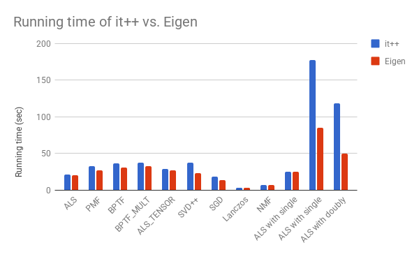
I am using Graphlab's collaborative filtering library, where the following algorithms are implemented:
ALS (alternating least squares), Tensor ALS (Alternating least squared on 3D tensor), PMF (probablistic matrix factoriation) , BPTF (Bayesian prob. tensor factorization), SVD++, NMF (non-negative matrix factorization), Lanczos algorithm, Weighted ALS, ALS with sparse factor matrices.
Each algorithm was tested once on top of it++ and a second time on Eigen, using a subset of Netflix data described here.
Following is a summary of the results:
* Installation: Eigen has no installation, since it is composed of header files. it++ has a problematic installation on many systems, since installation packages are available on only part of the platforms, and potentially BLAS and LaPaCK should bre preinstalled.
* Licensing: Eigen has LGPL3+ license, while it++ has a limiting GPL license.
* Compilation: Eigen compilation tends to be slower because of excessive template usage.
* Performance: Typically Eigen is slightly faster as shown in the graphs below.
* Accuracy: Eigen is more accurate when using ldlt() method (relative to it++ solve() method), while it++ performs better on some other problems, when using backslash() least squares solution.
Here is timing performance plot. Lower is running time is better.
Here is accuracy plot. Lower training RMSE (root square mean error) is better.

Overall, the winner is: Eigen - because of simpler installation, equivalent if not better performance and a more flexible license.
I am using Graphlab's collaborative filtering library, where the following algorithms are implemented:
ALS (alternating least squares), Tensor ALS (Alternating least squared on 3D tensor), PMF (probablistic matrix factoriation) , BPTF (Bayesian prob. tensor factorization), SVD++, NMF (non-negative matrix factorization), Lanczos algorithm, Weighted ALS, ALS with sparse factor matrices.
Each algorithm was tested once on top of it++ and a second time on Eigen, using a subset of Netflix data described here.
Following is a summary of the results:
* Installation: Eigen has no installation, since it is composed of header files. it++ has a problematic installation on many systems, since installation packages are available on only part of the platforms, and potentially BLAS and LaPaCK should bre preinstalled.
* Licensing: Eigen has LGPL3+ license, while it++ has a limiting GPL license.
* Compilation: Eigen compilation tends to be slower because of excessive template usage.
* Performance: Typically Eigen is slightly faster as shown in the graphs below.
* Accuracy: Eigen is more accurate when using ldlt() method (relative to it++ solve() method), while it++ performs better on some other problems, when using backslash() least squares solution.
Here is timing performance plot. Lower is running time is better.
Here is accuracy plot. Lower training RMSE (root square mean error) is better.
Overall, the winner is: Eigen - because of simpler installation, equivalent if not better performance and a more flexible license.
Subscribe to:
Posts (Atom)